 Last year the pension funds managed by CalPERS lost 23.5% of their value or $55 billion. At that point the largest fund was only 58.4% funded, well below the threshold of 80% which the CalPERS Board established in 2005 as the minimum level to be considered funded. CalPERS actuaries are taking the position the market sell-off was a onetime event and are amortizing the loss over 30 years.
Before his resignation, Dave Gilb, Personnel Administration Director and a CalPERS board member in a letter last June said the State’s contribution for 2010 including amortizing that loss would be $879 million. But in November, the CalPERS Board decided to postpone a decision and by early May of this year had settled on a $600 million increase in the contribution to $3.9 billion. Absent from that increase was the majority of the $879 million. $300 million of the increase is a result of an actuarial update showing a longer average life expectancy of State employees, $50 million is to cover earlier than anticipated retirements and $200 million was already anticipated because of earlier underfunding. ( The fund lost 5.8% between June of 2007 and June of 2008.) Instead, using a three year smoothing method that loads the largest contributions into the second and third years, the contribution made towards actually covering that loss will be around $115 million. There was a savings of $50 million from lower than anticipated salaries. Last week the CalPERS committee made it official and sent their recommendation to the board. A chart given to the CalPERS Board last spring showed that after the three year smoothing, contribution rates for most workers are expected to slowly climb for three decades, going from roughly 17 percent of payroll in 2012 to 27 percent by 2042. And the result is that by 2042 the plan will only be 76% funded.
The municipalities and agencies participating in CalPERS are a microcosm of the larger fund. The difference is they receive their actuarial adjustments a full year after the State and two years after changes in the fund occur. This has the effect of making people like me appear to cry wolf. It gives the municipal managers the ability to claim they are “fully funded” because by the definition of the actuaries at CalPERS they are. In fact they are two years behind.
The chronology of events leading up to this is pretty clear. In 1991 then Governor Pete Wilson signed legislation bringing the analysis and funding of CalPERS under the responsibility of the legislative and executive branches and reducing pension benefits. That was followed quickly in 1992 by a labor sponsored initiative, Proposition 162, approved by 51% of the voters, which returned control of the pension funds to the CalPERS actuaries. In 1999 CalPERS position was further strengthened and retirement benefits increased by SB 400, legislation written and sponsored by CalPERS and signed into law by Governor Grey Davis, which laid the groundwork for the now infamous 3% at 50 for safety employees.
Suffering from the collapse of the tech boom, in 2003 CalPERS lowered their assumed rate of return from 8.25% to 7.75% where it stands today but that created a problem. After the typical delays for actuarial calculations, by 2005 plans were underfunded so in 2005 the Board widened the band they consider funded from 90-110% to 80-120% giving cover to the plan managers in professing that their plans are “fully funded”. Today they are amortizing losses over longer periods of time, back loading payments required by their own actuarial assumptions and trying to correct their actuarial miscalculations.
For MMWD, and it seems consistent across most of the funds I look at, the elephant in the room is Other Post Employment Benefits or OPEBs, those other than direct pensions. There are two funds for pension liabilities. The first is direct pension payments which is on balance sheet and funded each year by the amount required by CalPERS. This is the contribution we are talking about today. Terry Stigall, the CFO of the MMWD told me last week this year’s contribution to the pension only part of the plan For MMWD will be 13.86% of covered salary or roughly $2.85 million. In addition they will make the entire employee contribution for senior managers of 8% and 3% of the 8% for all other employees bringing the total contribution to roughly 18% of covered payroll. The second fund is OPEBs which in the past was carried off balance sheet. Put in motion by the Government Accounting Standards Board Statement 45, beginning in 2009 municipal funds had to account for the future liability of OPEBs, something they had been simply funding on a cash basis before. In the Notes section of MMWD’s 2009 audited financials in reference to these liabilities it says, “As of January 1, 2007, the most recent actuarial valuation date, this plan was not funded. The actuarial accrued liability for benefits was $33,973,000, and the actuarial value of assets was $0.” In 2009 contributions to the two plans amounted to $7,408,610 or 39.3% of covered payroll and 12.66% of the total operating budget. This does not include Social Security, Medicare or any other taxes related to employment or any benefits associated with direct employment. Here is the schedule I got directly from MMWD.
 It demonstrates the effects of amortization of liabilities over 30 years. In unadjusted dollars the liability is actually higher after the first ten years than it was at the beginning. The payment for 2007-08 was not required and was not made and there appears to be no prevision for making it. The contribution for 2009-2010 will be $3.728 million. That means total contributions by MMWD for retirement benefits will equal about $7.928 million of a total estimated operating budget of $57 million or 13.9%. What is particularly of concern is that it is 1.2% higher as a percent of the total budget than it was last year and we haven’t even begun to deal with the losses incurred in the funds from the 2008-09 contraction!
In April of this year the Stanford Institute for Economic Policy Research published a report entitled, “Going for Broke: Reforming California’s Public Employee Pension Systems.” In it they argued the discount rate used in calculating the funded status of the three main pension funds managed by the public employee pension system is too high and the funds are in significantly worse shape than being reported. The discount rate is one of the inputs actuaries use in determining the funded status of plans. It is the assumed future returns of the plan. While there are a lot of variables; for example length of employment and lifespan of participants and their spouses, which apparently the actuaries have been getting wrong anyway, the two biggest variables are investment returns and inflation. The Stanford brief made the case taxpayers should not be responsible for miscalculations in fund returns or for inflation and therefore the investment rate should be the risk free rate and went so far as to suggest the use of TIPS, Treasury Inflation Protected Securities. In their argument against the assumptions used by the Stanford report CalPERS pointed to their historical returns. In the last 20 years these returns have averaged 7.91% and the number used by the actuaries for future returns is 7.75%.
On March 5 of this year an article appeared in the Wall Street Journal suggesting CalPERS may drop this rate to 6%. The result would cause an increase in unfunded liabilities by at least 15% as we saw in 2005.
So it would be reasonable to ask if these returns are achievable. In calculating their returns CalPERS uses 20 years. The only data available on historical fund returns I could find was from the annual reports posted on their web site and they only went back as far as 2002. Over that eight year period the average return was 3.44%. That means the average return for the twelve years leading up to 2002 had to be 15.5%. It also means that to achieve an average return of 7.75% for the period from 2002 to 2022 the next 12 years average also has to be 15.5%. I believe that will be quite a feat.

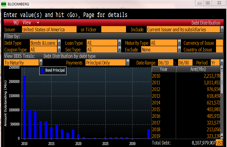
On April 7 they felt pretty good arguing against the Stanford brief. Year to date returns for the fund were 15.53%. However as you can see in the next panel by June 14, 2010 they were down over 4% leaving them with a return to date of 11.61%. And typically the largest returns, particularly in the stock market occur in the first year of recovery from a contraction. The Standard and Poor’s 500 is up 19.5% over that same time period.

I can almost hear the prayers for a quarter end rally before they close their year.
I would also put forth the proposition that the kinds of returns they anticipate over the next ten years are unachievable for several reasons.
- First, during the period from 1990 through 2001 US debt to GDP averaged 62%, the CBO forecasts debt to GDP to average 96% over the next eleven years (the twelfth year is not available but year eleven is the highest at 101% and increasing). The Bank for International Settlements (BIS) which is the international equivalent of the Federal Reserve, released a report in April entitled “The Future of Public Debt, Prospects and Implications” in which they make the case that once a country exceeds 90% debt to GDP they can expect GDP to be reduced by approximately 1% from what it might ordinarily be.
- Second, in their book “This Time Is Different” Carmen Reinhart and Kenneth Rogoff demonstrate how historically, severe contractions like we experienced in 2008 to 2009 are not easily overcome and the effects are around on average for ten years before reasonable economic growth reignites and that countries such as the US, with its high level of debt to GDP are inevitably forced to default on their debts either by devaluation or inflation before growth resumes.
- Finally the period when CalPERS achieved their superior returns was during a time there were significantly more employees paying in than taking out. Today the inflows are only slightly ahead of outflows and will turn negative before long. This is exactly what happened to the General Motors pension plans and brought General Motors down.

So the bottom line to me is this: if CalPERS is so confident they can achieve these returns and they can forecast the risk of inflation along with all the other variables associated with their actuarial shenanigans, why aren’t the public employees willing to take that risk instead of placing it on the backs of the rate payers and the taxpayers? You might agree but again Joseph Dear, the Chief Investment Officer of CalPERS weighs in, “…I might agree with the money managers, who tend to have a short-term investment horizon, that earnings may average 6% in the short term. But CalPERS has decades in which to repeat its past investment performance.”
Do they?


